Figure 1Description of the classification system. At stage I both radar and lidar measurements are performed (asynchronous). Stage II provides the lidar object list Ω^(t) and the processed radar measurement Ψ^(τ), which contains the range-Doppler-angle power spectrum. Using the timestamps, the measurements are matched at stage III and the ROIs are extracted from the power spectrum. At stage IV the ROIs are classified by the CNN.

Download

The concept of the classification system is depicted in Fig. 1. On the one hand, the lidar sensor is responsible for detecting objects and tracking them over time. It delivers at each time step t an object list Ω^(t). A single object $O_k^{\left(t\right)}$ within Ω^(t) is described by the tuple

where id_k is an identification number given to the k-th object, ts_k a time stamp of the measurement, x_k and y_k the estimated position (middle point of the estimated bounding box) in the car's coordinate system, and v_x,k and v_y,k the velocities in x and y direction.

On the other hand, the radar system is responsible for the object classification task. It is a chirp sequence frequency-modulated continuous wave radar with 8 receive channels. The channels are arranged as a uniform linear array in azimuth direction with neighboring elements separated by half a wavelength at 77 GHz. The back-scattered, down-converted, sampled signal at the receiver can be modeled by

with k the sample index within one chirp, l the chirp index, u the receiver index, f_B the beat frequency, f_D the Doppler frequency, f_θ the normalized spatial frequency, f_s the sampling frequency and T_c the chirp period (Pérez et al., 2018). By applying 3 independent fast Fourier transforms (FFTs) across the k, l and u axis the range-Doppler-angle spectrum is obtained. This allows to resolve objects in range, velocity and angle dimensions, depending on the system parameters shown in Table 1.

A radar measurement at time step τ is composed of the tuple

where P_B denotes the range-Doppler-angle power spectrum and “ts” the time stamp of the radar measurement.

Table 1Radar system configuration.

Download Print Version | Download XLSX

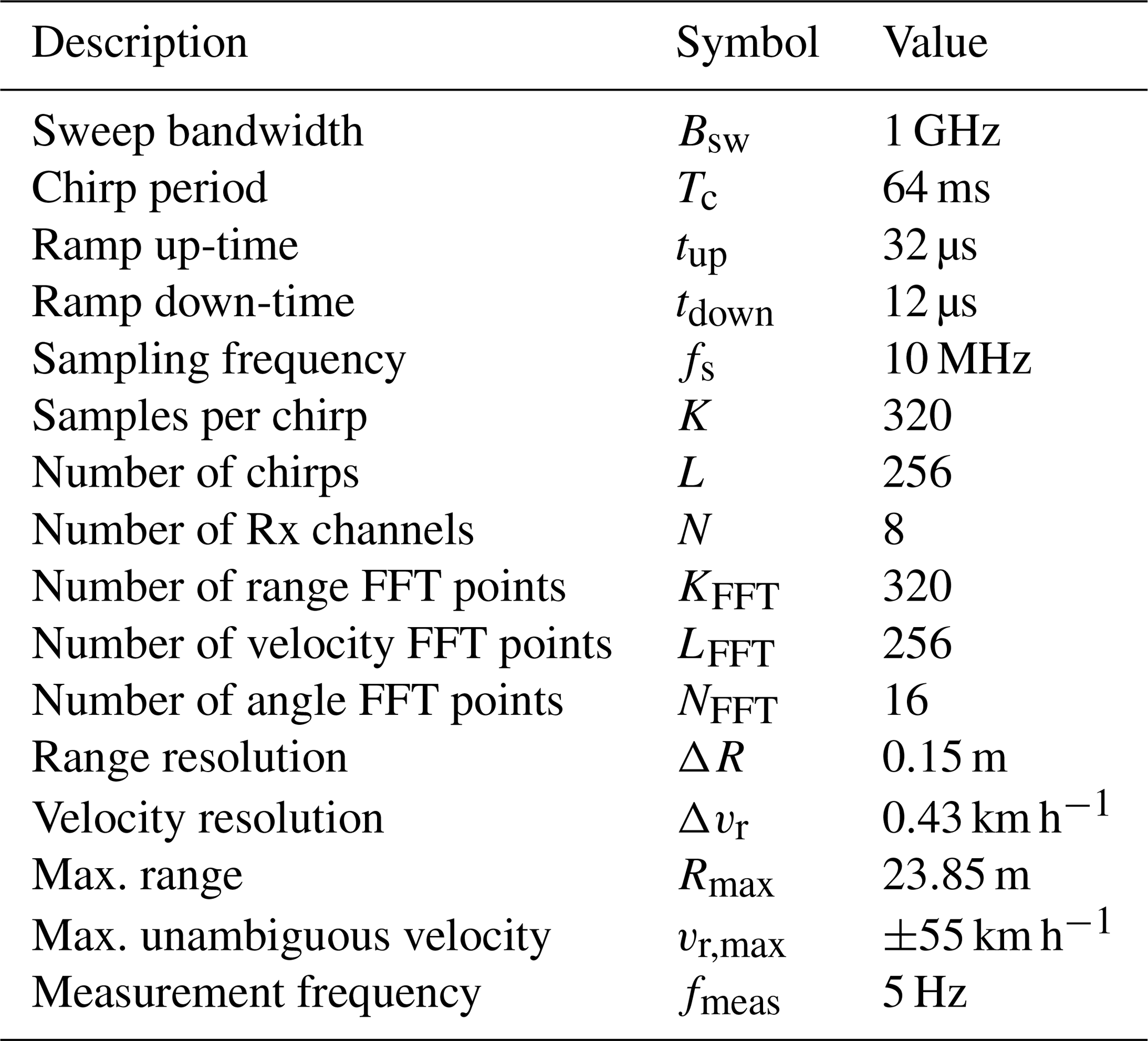
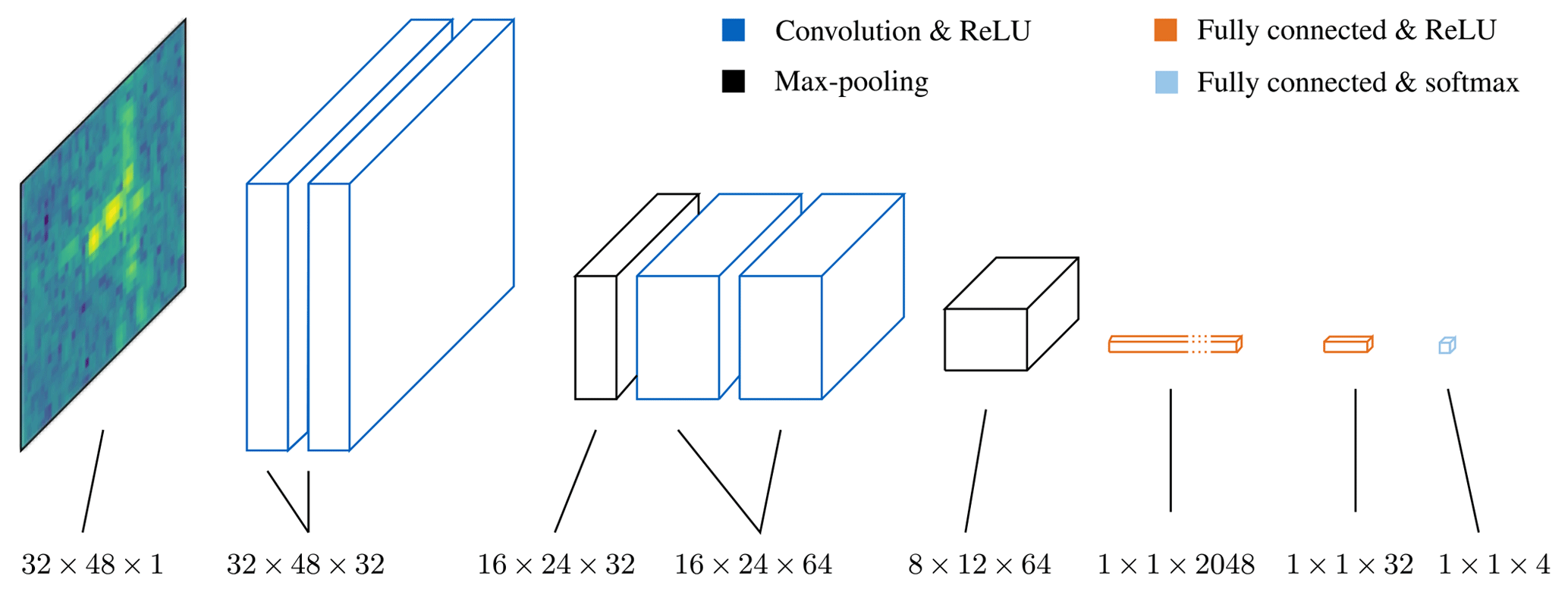
Figure 2Convolutional neural network architecture based on the VGGNet architecture from Simonyan and Zisserman (2014).

Since the lidar and radar measurements are not triggered by a common source, the measurements need to be matched to one another using their time stamps. The radar measurement frequency f_meas is the lower one and thus for each radar measurement a lidar measurement that best matches the radar's time stamp is selected.

After building a radar-lidar measurement pair, all the objects in Ω^(t) – excluding those outside the radar's field of view – are mapped to a location within the range-Doppler-angle power spectrum. This is achieved by converting an objects' spatial coordinates (x_k and y_k) to a range R_0,k and azimuth angle θ_k in the radar's coordinate system. In the same way, an object's radial velocity v_R,k and thus Doppler frequency is computed from its velocity components (v_x,k and v_y,k) provided by the lidar. A 2-dimensional region of interest (ROI) centered at (R_0,k, v_R,k) in range and Doppler dimensions is then extracted from $P_{\text{B}}^{\left(\mathit{\tau }\right)}$ at the azimuth angle bin nearest to θ_k (see Fig. 1 – III). The ROI is rectangular in shape and has a fixed size of $\mathrm{5}\text{m}\times \mathrm{20}{\text{km\hspace{0.17em}h}}^{-\mathrm{1}}$. This size was chosen to fit the range-Doppler signatures of pedestrians, bicycles and cars, while keeping it as small as possible.

Finally, the ROIs are fed to the convolutional neural network, which will be further explained in Sect. 2.1. The CNN computes the class probability vectors ${\mathit{P}}_{\text{class}}=[P_{\text{ped}},P_{\text{cyc}},P_{\text{car}},P_{\text{noise}}]$ and a decision is made in favor of the class with the highest probability.

To perform the measurements and acquire the data a test vehicle was used. The vehicle is a BMW 5 Series (F10) equipped with a variety of sensors. For this work only the radar, the front lidar and the front camera are of relevance (see Fig. 3). The radar system was fitted within the right kidney grill using a specially designed case. The front camera, mounted in place of the rear-view mirror, is exclusively used as an aid to label the radar data.

Figure 3Test vehicle (BMW 5 Series F10) equipped with radar (Radarbook from INRAS), lidar and camera sensors. Photograph source: [Authors].

The data was gathered by driving in the surrounding area of the Technical University of Munich. This resulted in a varied number of scenarios in real urban settings, i.e. subjects from all classes in a varied range of directions (both lateral and longitudinal with respect to the radar's orientation). All measurements were performed during daytime with no precipitation present.

In order to process the dataset the ROIs given by the lidar object lists were labeled semi-automatically and all frames were controlled and, if necessary, corrected manually. Since the classification approach produces one prediction per ROI, only tracks with one target present or with a clear dominant target within the ROI were selected. Figure 4 depicts an example measurement frame with the ROI enclosed by a red rectangle (upper half). The lower half of Fig. 4 displays the front camera picture, that shows a cyclist corresponding to the ROI.

The distribution of the training dataset can be taken from Table 2. A track T_id is composed of an arbitrary number of frames Z, which belong to the same object O_id:

where “id” stands for the object's identification number (see Eq. 1). In order to create the noise tracks, regions of the range-Doppler-angle power spectrum without any targets present were manually sampled. It is worth noting, that the car class includes larger vehicles, such as trucks, as well.

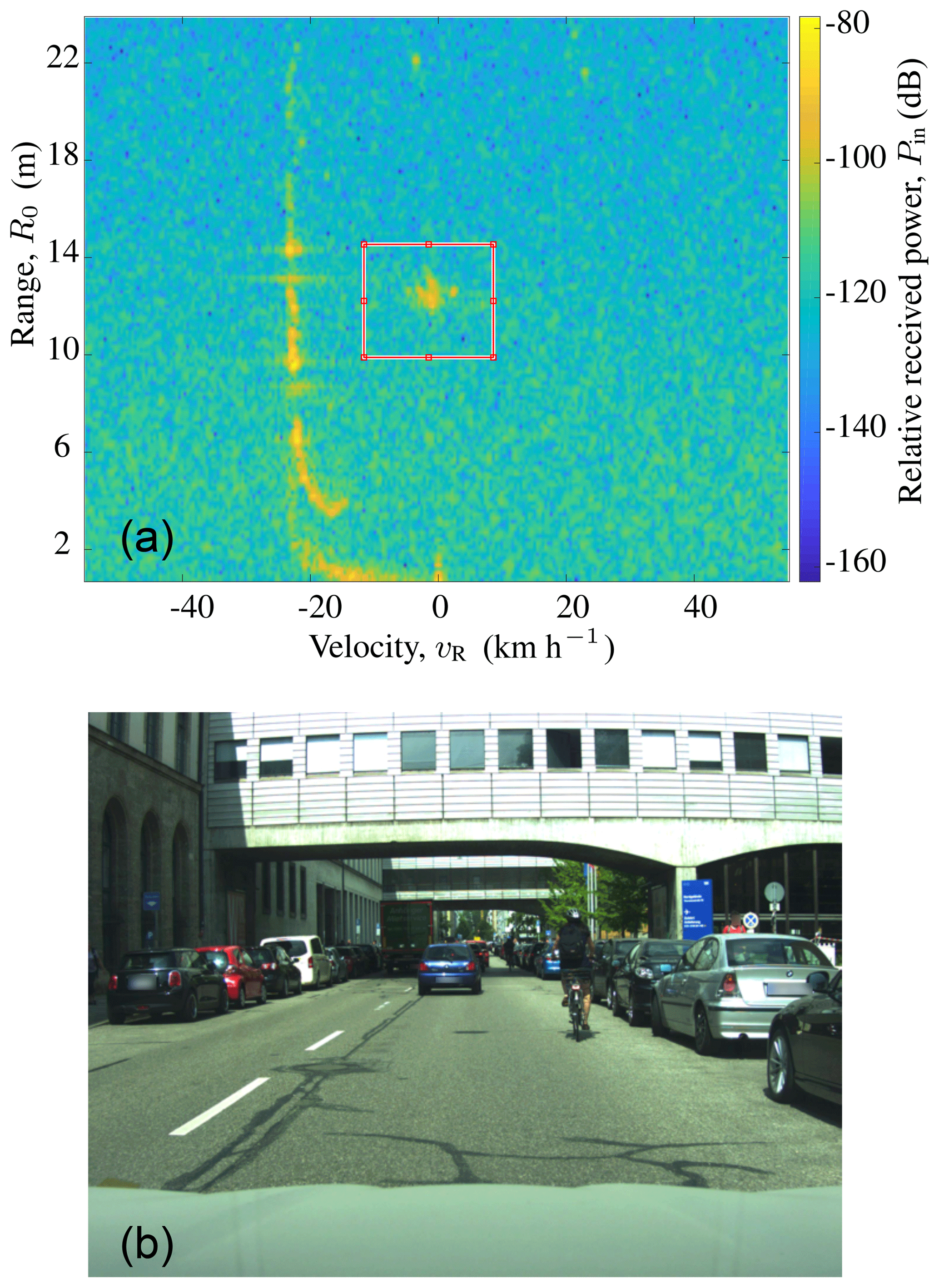
Figure 4Example of a measurement frame with a cyclist in the radar's FOV. The top half shows the range-Doppler-angle power spectrum P_B for a fixed angle with the ROI used for classification marked in red. The front camera picture is shown on the bottom half. Photograph source: [Authors].

The network was implemented with help of the TensorFlow software library (Abadi et al., 2015). Since the network is not particularly deep and the convolution filters are also quite small, training is not very time consuming. Using a NVIDIA GeForce GTX 1080 Ti GPU, the time it takes to train the CNN is only around 2 min. At test time, a single inference takes less than 2 ms (without taking into consideration any of the radar signal processing).

Table 2Distribution of the training dataset.

Download Print Version | Download XLSX

Table 3Distribution of the test dataset 1.

Download Print Version | Download XLSX

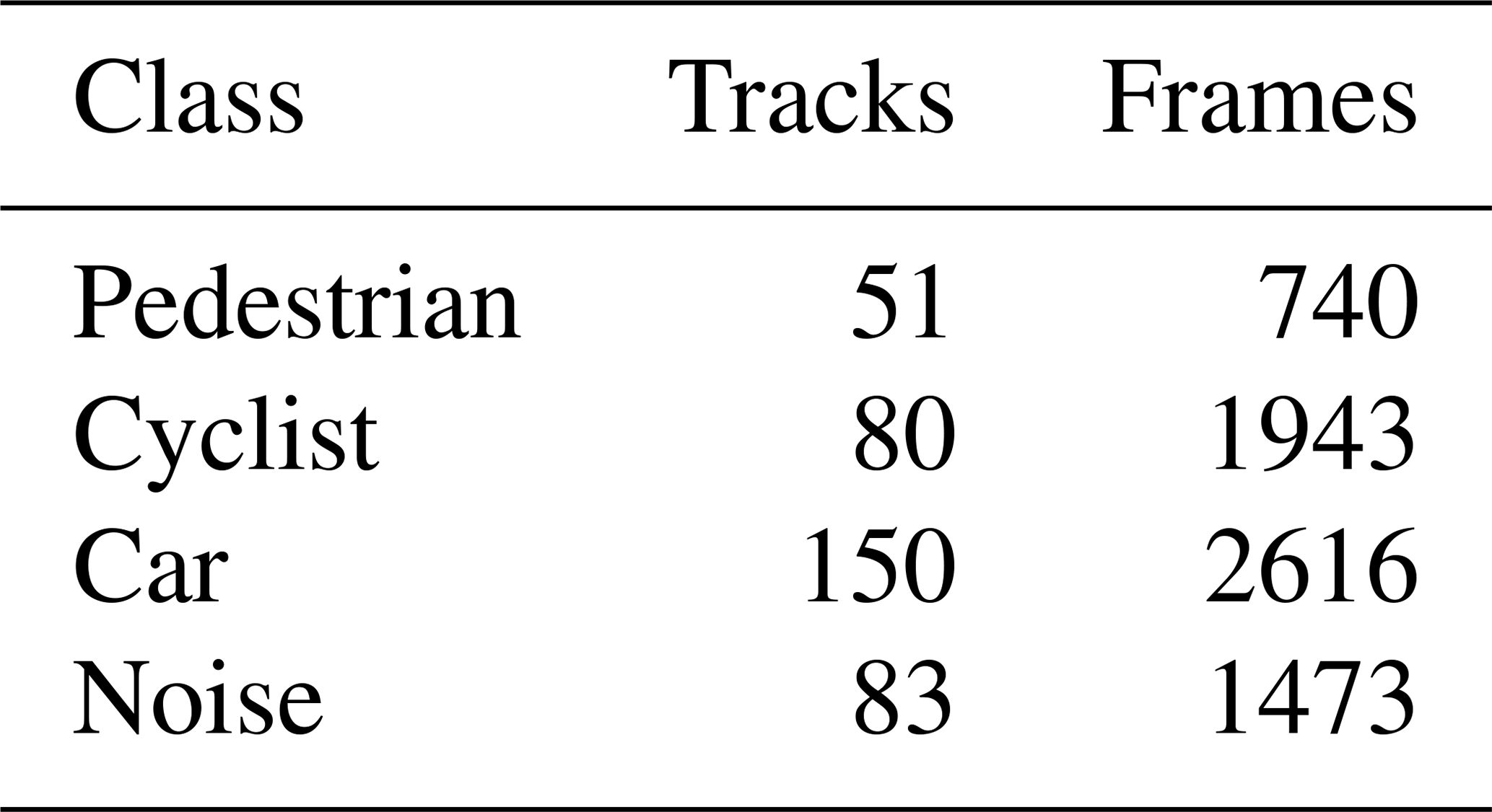
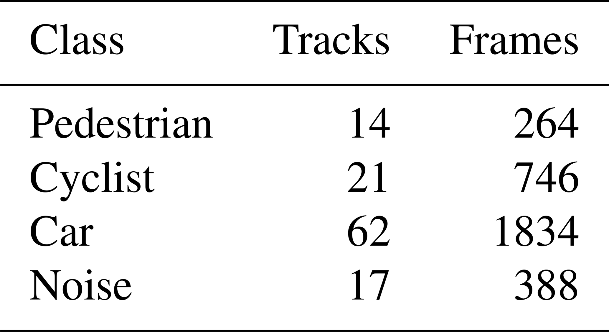
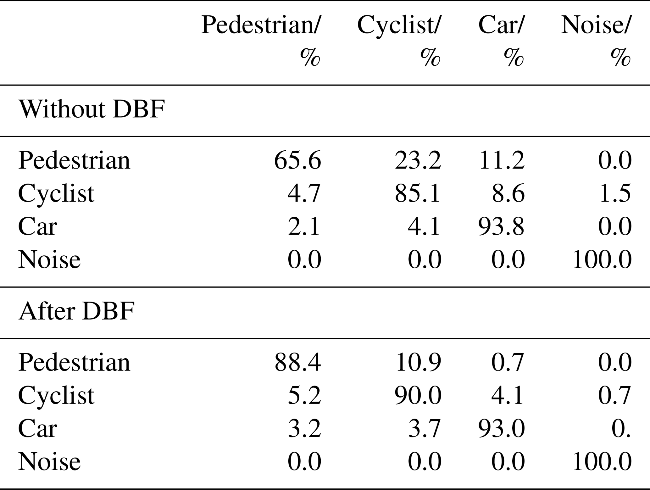
Table 4Confusion matrix for data set from Table 3 before (top) and after (bottom) DBF.

Download Print Version | Download XLSX

Table 5Precision and recall for data set from Table 3 before (top) and after (bottom) DBF.

Download Print Version | Download XLSX

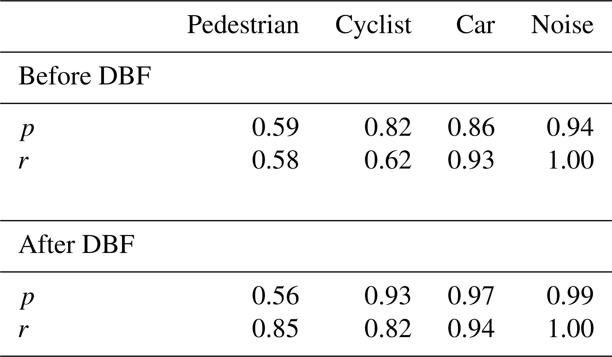
The top half of Table 4 shows the confusion matrix that results after running the data set from Table 3 through the convolutional neural network. Two common metrics to assess the performance of a classifier are the precision and the recall. The precision is defined as

where “tp” is the number of true positives and “fp” the number of false positives. It relates the number of correct predictions (tp) to the number of overall positive predictions (tp+fp) for a given class. On the other hand, the recall, or sensitivity, gives the fraction of a class that gets correctly classified and it is defined as

where “fn” is the number of false negatives (Shalev-Shwartz and Ben-David, 2014, p. 244).

From both the precision and the recall it can be seen that the classification network has trouble with the pedestrian class. A glance at the confusion matrix (top half of Table 4) shows that pedestrians tend to be confused with both cyclists and cars. While the classifier performs better for cyclists, about a third of all cyclist frames get wrongfully classified as cars. The car and noise classes show an overall good performance with the car class having just a small percentage misclassified as either pedestrians or cars. The overall classification accuracy for this data set is 0.84.

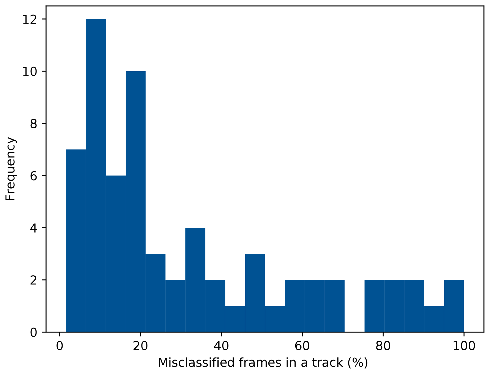
Figure 5Histogram of the relative number of erroneously classified frames per track. Tracks without any misclassified frames are not included.

Download

A further analysis of the results shows, that many classification errors occur for only a small number of frames within a track. Figure 5 depicts a histogram of the relative number of errors per track (excluding tracks without errors). From the histogram it can be observed, that tracks with a low percentage of misclassified frames are more frequent than tracks with a high percentage of misclassified frames.

Nonetheless, there are still tracks where the system fails to correctly classify the majority of the frames (15 out of 114 tracks). One common occurrence that can be observed within some of these tracks (5 out of 15) is multiple objects falling inside the ROI. While most tracks with multiple objects within an ROI were sorted out during labeling, tracks where it was assessed that the object of interest was visible enough were still allowed. Figure 6 depicts such an example, where 2 cyclists are riding closely together. The system erroneously classifies this track as a car for most of its lifetime. The same happens in other tracks, where e.g. pedestrians are crossing the street in groups, or when a pedestrian is walking slowly near parked cars. This highlights an inherent weakness of the approach, namely that of overlapping targets, since the train set contains mainly frames where only one single target is present in the ROI.

4.1 Filtering the classifications

By applying a high level filter on top of the classifier, the classification performance could be improved, since tracks with small percentages of misclassified frames (the majority) would tend to 0 % misclassifications. Nonetheless, tracks with big percentages of misclassified frames will tend to even higher percentages, but since they are the minority, an overall improvement would be achieved.

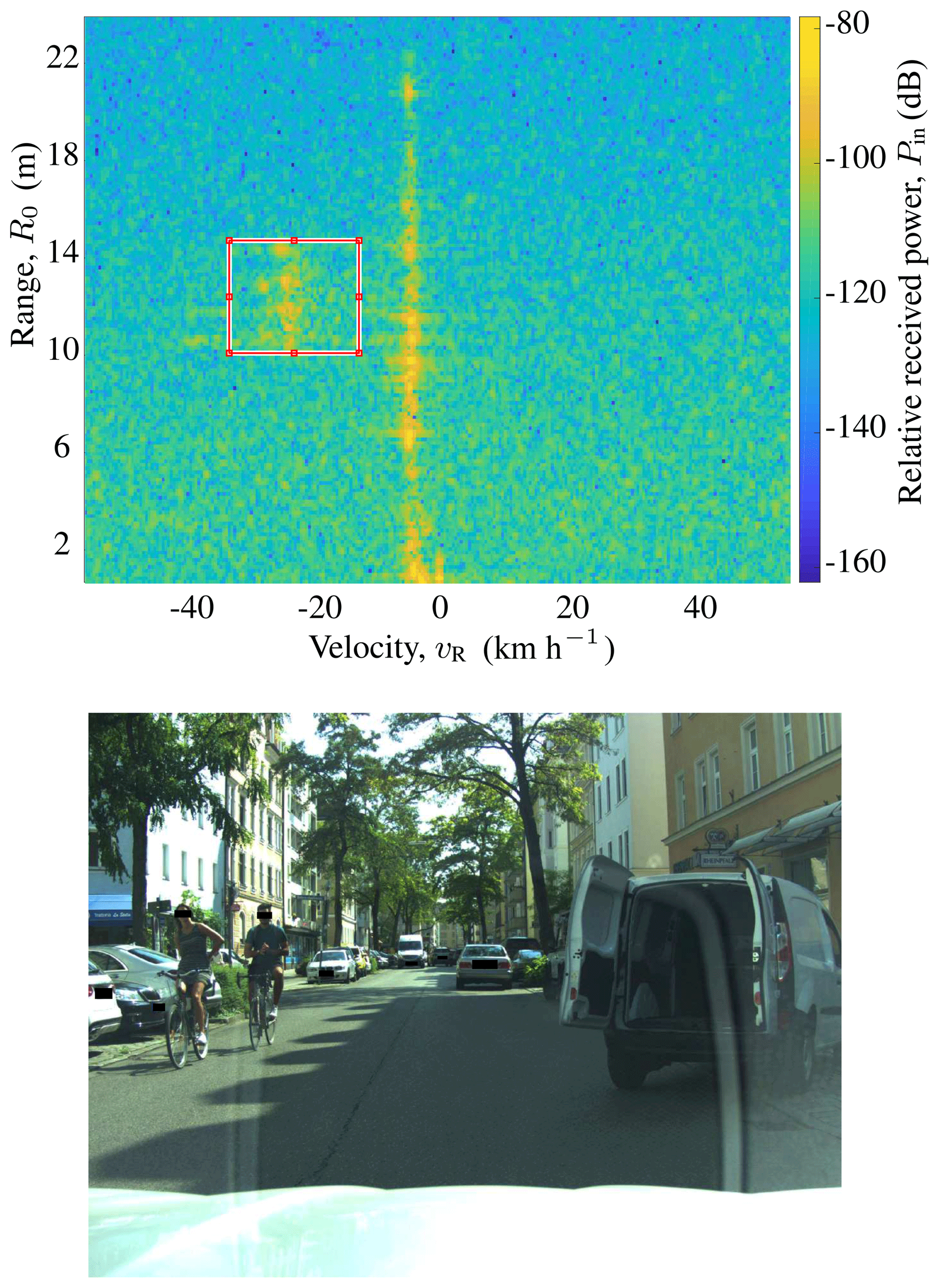
Figure 6Exemplary frame, where two bicycles fall within one single ROI, which leads to a high percentage of misclassified frames within the track. Photograph source: [Authors].

For this purpose a discrete Bayes filter (DBF) was chosen. An object is modeled as a random state variable X and the four classes (pedestrian, cyclist, car and noise) represent the discrete states x_c that X can take on. The goal of a DBF is to recursively estimate at time t the discrete posterior probability distribution

$$\begin{array}{}\text{(7)}& \left\{p_{\mathrm{c},t}\right\}=\left\{p\left(X_t=x_{\mathrm{c}}|z_{\mathrm{1}:t}\right)\right\},c=\mathrm{1}\mathrm{\dots }\mathrm{4}\end{array}$$

where z_1 : t stands for all measurements up to time t, by assigning a probability p_c,t to each of the single states. The working principle of the DBF can be taken from Algorithm Discrete Bayes filter. Adapted from p. 87. Require: {pc,t-1},zt for all c do p‾c,t=∑ip(Xt=xc|Xt-1=xi)pi,t-1=pc,t-1 pc,t=ηp(zt|Xt=xc)p‾c,t end for return  {pc,t} (Thrun et al., 2005). For a single object at time t the function loops over all four possible states (classes) x_c and computes their respective probability p_c,t. To do this, first the so called prediction, or prior, ${\stackrel{\mathrm{‾}}{p}}_{\mathrm{c},t}$ is calculated in line 2. The term $p(X_t=x_{\mathrm{c}}|X_{t-\mathrm{1}}=x_i)$ is called the state transition probability and it represents the probability of going from state x_i at time t−1 to state x_c at time t. Here it is assumed that an object cannot change classes during its lifetime. Therefore, it follows that

$$\begin{array}{}\text{(8)}& p\left(X_t=x_{\mathrm{c}}|X_{t-\mathrm{1}}=x_i\right)=\left\{\begin{array}{ll}\mathrm{1},& \text{if }{x}_{\mathrm{c}}=x_i\\ \mathrm{0},& \text{otherwise}\end{array}\right.\end{array}$$

and thus ${\stackrel{\mathrm{‾}}{p}}_{\mathrm{c},t}=p_{\mathrm{c},t-\mathrm{1}}$. In line 3 the current measurement z_t is incorporated by multiplying its likelihood $p\left(z_t\right|X_t=x_{\mathrm{c}})$ with the prior. The measurement z_t at time t corresponds to the class with the highest probability as predicted by the CNN and its likelihood $p\left(z_t\right|X_t=x_{\mathrm{c}})$ is derived from the statistics given by the confusion matrix in the top half of Table 4. Since the product $p\left(z_t\right|X_t=x_{\mathrm{c}}){\stackrel{\mathrm{‾}}{p}}_{\mathrm{c},t}$ is usually not a probability, a normalization factor η makes sure that the sum of all p_c,t add up to one and thus, that {p_c,t} is a probability distribution. When a new track is started, the DBF needs an initial probability distribution $p_{\mathrm{c},t=\mathrm{0}}$ to compute the first estimate. Since no knowledge about the initial state is assumed, a uniform distribution is assigned to it.

Discrete Bayes filter. Adapted from Thrun et al. (2005, p. 87).

• Require:

  1$\mathit{\left\{}{p}_{\mathrm{c},t-\mathrm{1}}\mathit{\right\}},z_t$

• 2for all c do

  • 3${\stackrel{\mathrm{‾}}{p}}_{\mathrm{c},t}={\sum }_{i}p(X_t=x_{\mathrm{c}}|X_{t-\mathrm{1}}=x_i)p_{i,t-\mathrm{1}}=p_{\mathrm{c},t-\mathrm{1}}$

  • 4$p_{\mathrm{c},t}=\mathit{\eta }p\left(z_t\right|X_t=x_{\mathrm{c}}){\stackrel{\mathrm{‾}}{p}}_{\mathrm{c},t}$

• 5end for

• 6return  {p_c,t}

The results from applying the discrete Bayes filter can be taken from the bottom half of Table 4. The confusion matrix clearly shows an improvement of the classification accuracy for all classes. From the bottom half of Table 5 the precision and recall after applying the DBF can be seen. A substantial improvement of the recall for both pedestrian and cyclist classes is observed. A histogram of the relative number of errors per track after incorporating the DBF is also shown in Fig. 7. It can be seen that one clear drawback of this approach is that the number of completely misclassified tracks increases. These are the tracks that already had a high percentage of misclassified frames to begin with. Still, the overall classification accuracy improves from 0.84 to 0.91 after applying the DBF.

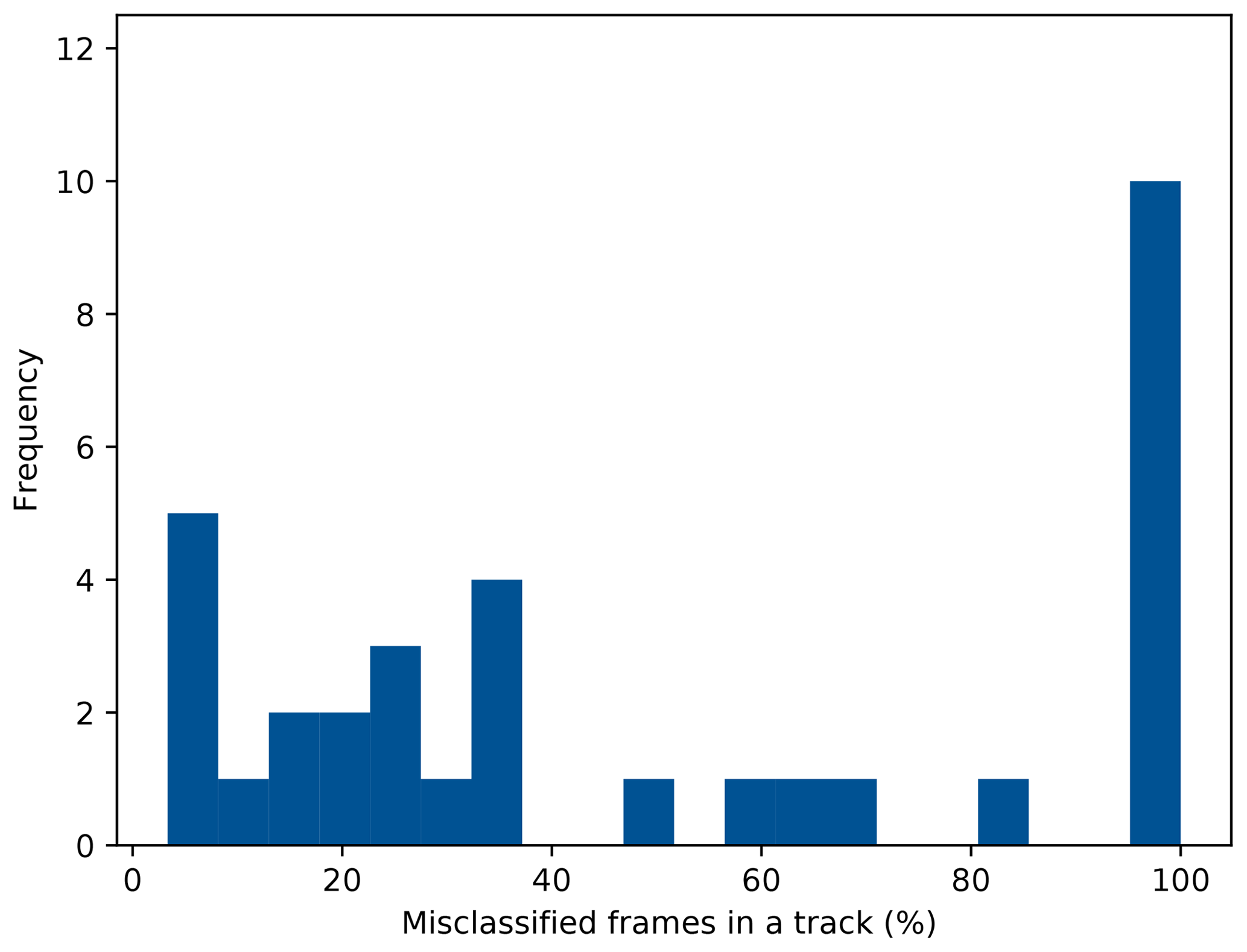
Figure 7Histogram of the relative number of erroneously classified frames per track after the discrete Bayes filter. Tracks without any misclassified frames are not included.

Download

Since the likelihood values needed for the DBF were taken from the confusion matrix on Table 4, a new set of measurements is needed to make sure that the proposed filter doesn't only work with that specific dataset. A different set of data (see Table 6) was used to evaluate again the improvement after applying the DBF. The results for this set are laid out on Table 7. It is evident, that the filter improves the overall classification performance for this data set as well. In this case the overall accuracies are 0.91 before and 0.94 after the DBF.

Table 6Distribution of the test dataset 2.

Download Print Version | Download XLSX

Table 7Confusion matrix for new data before (top) and after (bottom) DBF.

Download Print Version | Download XLSX

The data used in this paper is available upon request.

RP developed the concept, gathered the data and evaluated the performance of the system. RP prepared the manuscript with feedback from FS, RR and EB. FS, RR and EB supervised the project and provided resources.

The authors declare that they have no conflict of interest.

This article is part of the special issue “Kleinheubacher Berichte 2018”. It is a result of the Kleinheubacher Tagung 2018, Miltenberg, Germany, 24–26 September 2018.

This work was supported by the German Research Foundation (DFG) and the Technical University of Munich (TUM) in the framework of the Open Access Publishing Program.

This paper was edited by Jens Anders and reviewed by two anonymous referees.