It is well known that the solution of Maxwell's partial differential equation can be reduced to the determination of a vector and a scalar potential. In 1889, Hertz showed that it is possible to define an electromagnetic field with a single vector function (Hertz, 1889). Such a vector function, called the Hertz vector, is simply related to the vector and scalar potential if the region is restricted to an isotropic and homogeneous medium within which are no conduction currents or free electric charges $\left(\mathit{J}=\mathbf{0},\mathit{\rho }=\mathrm{0}\right)$. As a matter of fact, the Hertz vector is only one possible approach. There are two types, the electric and magnetic type (Π_E,Π_M), both satisfying the same vector Helmholtz equation of the form

In general, the vector Helmholtz Eq. (1) is still too complicated for an analytic solution (Moon and Spencer, 1952). Therefore, it is necessary to take appropriate simplifying steps, so that a particular solution can be easily determined without mathematical difficulties. As common in waveguide analysis, we introduce orthogonal circular curvilinear coordinates $(u,v,z)$, with metrical coefficients $(h_u,h_v,h_z)$. In the case of straight and uniform waveguides, the metrical coefficients of the relevant coordinate system satisfy (Huang and Hung-Chia, 1984)

Thus, in a source free region, the boundary problem is reduced to solving the scalar 2-dimensional Helmholtz equation, which together with the appropriate boundary condition associated with the differential equation is satisfied by the longitudinal component of the Hertz vector

The reduction of the vector Helmholtz Eq. (1) to the scalar Helmholtz Eq. (3) is a significant step in simplifying the mathematics. For the sake of brevity, we use Π to represent ${\mathrm{\Pi }}_{\mathrm{E},z},{\mathrm{\Pi }}_{\mathrm{M},z}$. In the following we will use the method of separation of variables, we assume

where W(z) is a function of the longitudinal coordinate and ${\mathrm{\Pi }}_{\perp }\left(u,v\right)$ a function of the transverse coordinates. The separation of variables yields

in which $k_z^{\mathrm{2}}=k^{\mathrm{2}}-k_{\perp }^{\mathrm{2}},k^{\mathrm{2}}:={\mathit{\omega }}^{\mathrm{2}}\mathit{\mu }\mathit{\epsilon }$. It is apparent that the second Eq. (5) has solutions of the form exp (±k_zz), representing forward and backward traveling waves in the longitudinal direction. The transverse pattern of these waves is described independently by the solutions of the 2-dimensional Helmholtz equation. Once Π is found, the electromagnetic field can be derived by simple differentiation according to (Stratton, 1941)

The concept of the so-called generalized telegraphist's equations starts with the separation of the electromagnetic field components and Nabla operator

where ${\mathit{E}}_{⟂},{\mathit{H}}_{⟂}$ are the transverse and E_z,H_z are the longitudinal components of the total field. The time dependence exp (−jωt) is omitted. Substituting these fields into the source free Maxwell's equation, we obtain

for the transvers fields and

for the longitudinal components. In the next step, the transverse field components will be expanded into series of orthogonal functions of the following form

in which ${\mathit{e}}_{\mathrm{M},n},{\mathit{h}}_{\mathrm{M},n}$ are the vector fields of the eigenmodes of the TM-mode, while those with the index E refer to the eigenmodes of the TE-mode (Reiter, 1959). There are various approaches to the expansion of the electromagnetic field components. A more detailed treatment of the field expansion can be found in the work of Huang and Hung-Chia (1984). The coefficients V_n,I_n are called the complex voltage and current amplitudes. It should be mentioned that the physical dimensions of the coefficients are not those of voltage and current. The eigenmodes are simply related to the previously mentioned Hertz functions (Huang and Hung-Chia, 1984)

These vector functions e_n,h_n have certain orthogonality properties which can be expressed as

The Hertz functions of the various modes are determined by Eq. (5) and the boundary conditions Eq. (3) except for arbitrary factors related to the power of the modes. If we choose these constants in such a way that

where S is the cross-section of the waveguide, then the complex power carried by the modes is described by (Schelkunoff, 1952)

In this case, the complex voltage and current coefficients correspond to voltages and currents. In order to derive the GTE's, the series expansion Eq. (10) of the transverse field will be substituted into the Eqs. (8) and (9). Subsequently, these equations will be multiplied with orthogonal functions and integrated over the waveguide cross-section 𝒮. Using the orthogonal condition Eq. (13) (Schelkunoff, 1952) and Green's second identity (Schelkunoff, 1951), the GTE's for the basis coeffcients V_n,I_n of the series expansion of the TM- and TE-Modes are derived

The set of GTE's is equivalent to the equations in Unger (1961b). A more detailed derivation of the equation above can be found in Weiss and Mathis (1998). For a further analysis of the GTE's, the field components in the integral kernel of the line integral need to be determined.

2.1 Boundary Conditions

There are different kinds of boundary conditions to model the actual boundary of a waveguide. One of the most commonly used boundary conditions is the perfect electric conductor (PEC)

$$\begin{array}{}\text{(18)}& {\displaystyle }\mathit{n}\times \mathit{E}=\mathbf{0},\mathit{n}\cdot \mathit{B}=\mathrm{0},\mathit{n}={\displaystyle \frac{\frac{\partial \mathit{r}}{\partial \mathit{\varphi }}\times \frac{\partial \mathit{r}}{\partial z}}{\left|\frac{\partial \mathit{r}}{\partial \mathit{\varphi }}\times \frac{\partial \mathit{r}}{\partial z}\right|}}.\end{array}$$

where n is the outward unit normal vector to the boundary ∂𝒮. In case of a circular waveguide, we obtain of Eq. (18) for the tangential electric and normal magnetic components

$$\begin{array}{}\text{(19)}& {\displaystyle }{\left.E_{\mathit{\varphi }}\right|}_{\partial \mathcal{S}}=\mathrm{0},{\left.E_z\right|}_{\partial \mathcal{S}}=\mathrm{0}\text{and}{\left.B_r\right|}_{\partial \mathcal{S}}=\mathrm{0}.\end{array}$$

The equations above specify the relations which must be satisfied by the electric and magnetic field at the boundary ∂𝒮.

In case of small irregular deformations of the cross-section, it is appropriate to use the perturbation theory. The surface of the waveguide can be represented in cylindrical coordinates $\left(r,\mathit{\varphi },z\right)$. The radius r of the cross-section is a function of ϕ,z and a parameter ω

$$\begin{array}{}\text{(20)}& {\displaystyle }r\left(\mathit{\xi }\left(\mathit{\varphi },z,\mathit{\omega }\right)\right)=r_{\mathrm{0}}\cdot \left(\mathrm{1}+\mathit{\xi }\left(\mathit{\varphi },z,\mathit{\omega }\right)\right),\end{array}$$

where r₀ is the waveguide mean radius and the function ξ describes the irregular deformation of the cross-section. For convenience the deformation function ξ will only be a function of ϕ and ω. So instead of the usual boundary conditions Eq. (19), the field components have additional terms

$$\begin{array}{}\text{(21)}& {\displaystyle }{E}_{\mathit{\varphi }}=\mathrm{0},E_z={\displaystyle \frac{\partial r(\mathit{\varphi },\mathit{\omega })}{\partial \mathit{\varphi }}}{E}_r\text{and}{B}_r={\displaystyle \frac{\partial r(\mathit{\varphi },\mathit{\omega })}{\partial \mathit{\varphi }}}{B}_{\mathit{\varphi }}.\end{array}$$

The next task is to express the field components at a mean surface r₀ (regular boundary) and this is done by expanding the field components in a Taylor series in ξ (Senior, 1960; Unger, 1961a). Since the field is finite and continuous within the boundary, we have the following form

$$\begin{array}{}\text{(22)}& \begin{array}{ll}{E}_{\mathit{\varphi }}(r\left(\mathit{\xi }\right),\mathit{\varphi })& =E_{\mathit{\varphi }}(r_{\mathrm{0}},\mathit{\varphi })+r_{\mathrm{0}}\mathit{\xi }{\displaystyle \frac{\partial }{\partial r}}{E}_{\mathit{\varphi }}(r_{\mathrm{0}},\mathit{\varphi })\\ & +r_{\mathrm{0}}^{\mathrm{2}}{\displaystyle \frac{{\mathit{\xi }}^{\mathrm{2}}}{\mathrm{2}}}{\displaystyle \frac{{\partial }^{\mathrm{2}}}{\partial r^{\mathrm{2}}}}{E}_{\mathit{\varphi }}(r_{\mathrm{0}},\mathit{\varphi })+\mathrm{\dots },\end{array}\end{array}$$

where the differentiation must be carried out before r is put equal to r₀. In this paper, we will use the first order approximation of the boundary condition and all higher order terms will be neglected (Unger, 1961a). Substituting the Taylor series into Eq. (21), we obtain

$$\begin{array}{}\text{(23)}& \begin{array}{ll}{\left.E_{\mathit{\varphi }}\right|}_{\partial \mathcal{S}}& =-r_{\mathrm{0}}\mathit{\xi }{\displaystyle \frac{\partial E_{\mathit{\varphi }}}{\partial r}},\\ {\left.E_z\right|}_{\partial \mathcal{S}}& ={\displaystyle \frac{\partial r(\mathit{\varphi },\mathit{\xi })}{\partial \mathit{\varphi }}}\left(E_r+r_{\mathrm{0}}\mathit{\xi }{\displaystyle \frac{\partial E_r}{\partial r}}\right)-r_{\mathrm{0}}\mathit{\xi }{\displaystyle \frac{\partial E_z}{\partial r}},\\ {\left.B_r\right|}_{\partial \mathcal{S}}& ={\displaystyle \frac{\partial r(\mathit{\varphi },\mathit{\xi })}{\partial \mathit{\varphi }}}\left(B_{\mathit{\varphi }}+r_{\mathrm{0}}\mathit{\xi }{\displaystyle \frac{\partial B_{\mathit{\varphi }}}{\partial r}}\right)-r_{\mathrm{0}}\mathit{\xi }{\displaystyle \frac{\partial B_r}{\partial r}}.\end{array}\end{array}$$

For a more general approach the IBC will be used (Katsenelenbaum, 1998)

$$\begin{array}{}\text{(24)}& \mathit{n}\times \mathit{E}=Z\cdot \mathit{n}\times \left(\mathit{n}\times \mathit{H}\right),Z={\displaystyle \frac{k}{\mathit{\kappa }-\mathrm{j}\mathit{\mu }\mathit{\epsilon }}}.\end{array}$$

It can be shown that the PEC Eq. (18) is only a special case of the IBC Eq. (24) (Z=0). Using the same method as above, we obtain two equations for the tangential electric field components

$$\begin{array}{}\text{(25)}& \begin{array}{ll}{E}_z& =Z\cdot \left(H_{\mathit{\varphi }}+{\displaystyle \frac{\partial r(\mathit{\varphi },\mathit{\xi })}{\partial \mathit{\varphi }}}{H}_r\right),\\ E_{\mathit{\varphi }}& =-Z\left(H_z+{\left({\displaystyle \frac{\partial r(\mathit{\varphi },\mathit{\xi })}{\partial \mathit{\varphi }}}\right)}^{\mathrm{2}}{H}_z\right)-{\displaystyle \frac{\partial r(\mathit{\varphi },\mathit{\xi })}{\partial \mathit{\varphi }}}{E}_{\mathit{\varphi }},\end{array}\end{array}$$

which can be substituted in the line integral of Eqs. (16) and (17).

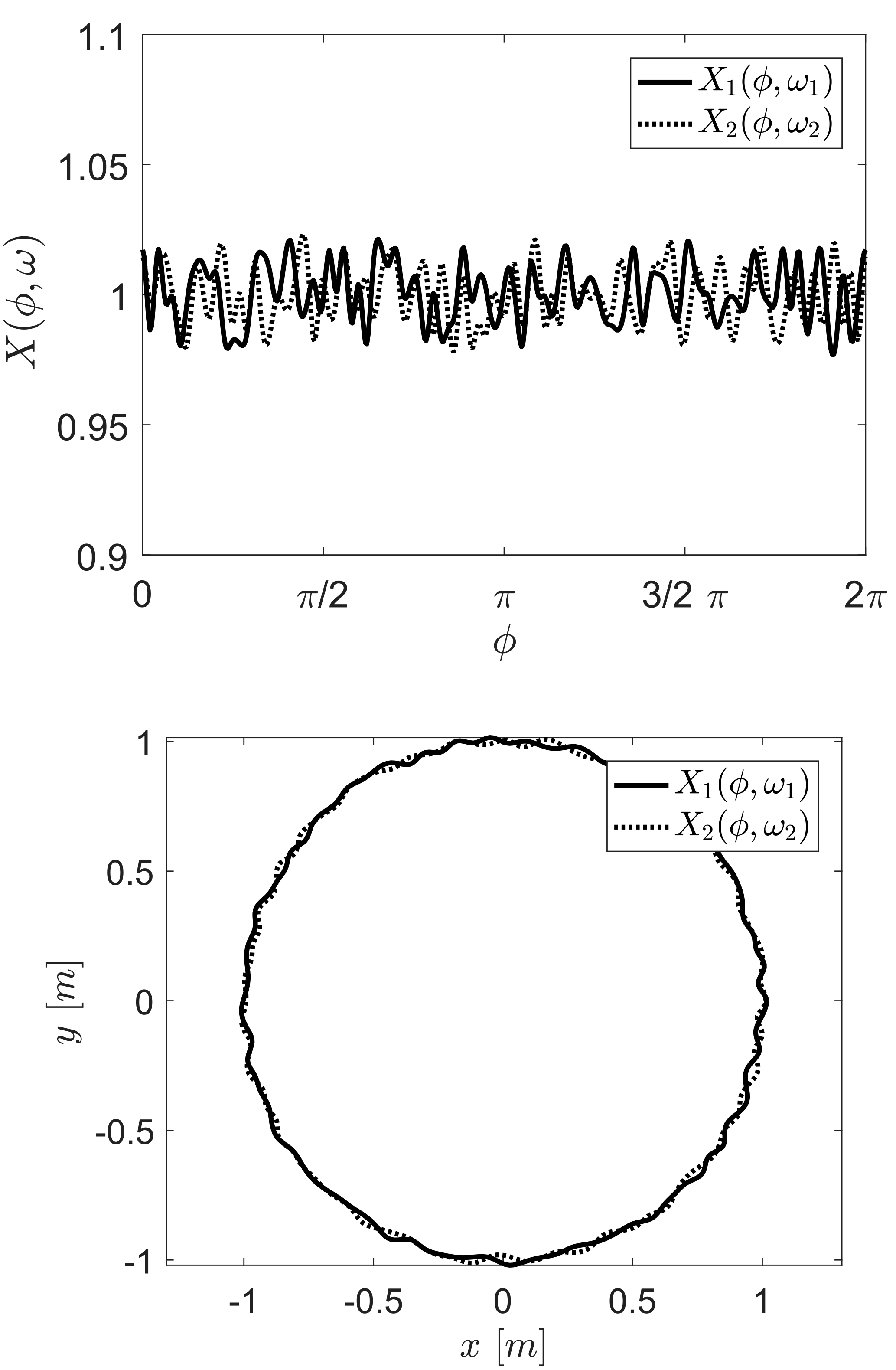
Figure 1X₁(ϕ,ω₁) and X₂(ϕ,ω₂) are two realizations of the stochastic process. Parameters for simulations: N=60, r₀=1 and ${\mathit{\delta }}_{max}=\mathrm{1}$.

Download

2.2 Stochastic Process

In the previous section, the boundary condition for an irregular deformed waveguide was modeled. The imperfections on the surface ∂S, where we assume that there is no rule for these deformations, were described by the function ξ(ϕ,ω). Therefore, it is useful to interpret the perturbation term ξ as a random variable X(ϕ,ω). For this purpose, an appropriate probability space $(\mathrm{\Omega },\mathcal{A},P)$ with a sample space Ω, a σ-algebra 𝒜 and a probability measure P has to be constructed where ω∈Ω (Mathis and Mathis, 2015). For computational and mathematical reasons, the stochastic process has the following form

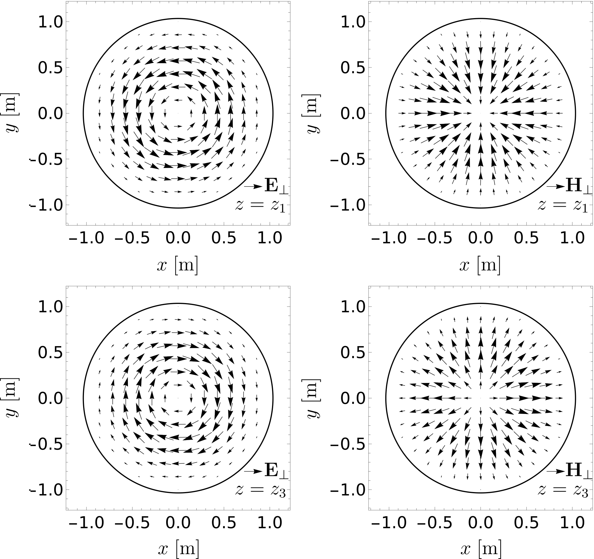
Figure 2Change of transverse field pattern of the electric and magnetic field along the z-axis.Parameters for simulation: N=60, r₀=1 and ${\mathit{\delta }}_{max}=\mathrm{0.1}$.

Download

Table 1Coupling modes in the irregularly deformed waveguide.

Download Print Version | Download XLSX

$$\begin{array}{ll}{\displaystyle }& {\displaystyle }X\left(\mathit{\varphi },\mathit{\omega }\right)=\\ \text{(26)}& {\displaystyle }& {\displaystyle }\begin{array}{l}\left\{\begin{array}{lcl}{\mathit{\xi }}_{\mathrm{1}}\left(\mathit{\varphi },\mathit{\omega }\right),& \mathrm{0}\le \mathit{\varphi }\le {\displaystyle \frac{\mathrm{2}\mathit{\pi }}{N}},& \mathit{\omega }\in \mathrm{\Omega }\\ \mathrm{⋮}& \mathrm{⋮}& \mathrm{⋮}\\ {\mathit{\xi }}_n\left(\mathit{\varphi },\mathit{\omega }\right)& {\displaystyle \frac{\mathrm{2}\mathit{\pi }\left(n-\mathrm{1}\right)}{N}}<\mathit{\varphi }\le {\displaystyle \frac{\mathrm{2}\mathit{\pi }n}{N}}& \mathit{\omega }\in \mathrm{\Omega }\\ \mathrm{⋮}& \mathrm{⋮}& \mathrm{⋮}\\ {\mathit{\xi }}_N\left(\mathit{\varphi },\mathit{\omega }\right),& {\displaystyle \frac{\mathrm{2}\mathit{\pi }\left(N-\mathrm{1}\right)}{N}}<\mathit{\varphi }\le \mathrm{2}\mathit{\pi },& \mathit{\omega }\in \mathrm{\Omega }\end{array}\right.\end{array}\end{array}$$

with

$${\mathit{\xi }}_n=c_{n,\mathrm{3}}\left(\mathit{\omega }\right)\cdot {\mathit{\varphi }}^{\mathrm{3}}+c_{n,\mathrm{2}}\left(\mathit{\omega }\right)\cdot {\mathit{\varphi }}^{\mathrm{2}}+c_{n,\mathrm{1}}\left(\mathit{\omega }\right)\cdot \mathit{\varphi }+c_{n,\mathrm{0}}\left(\mathit{\omega }\right).$$

With this specific form of the stochastic process X(ϕ,ω), the randomness is contained in the coefficients c_n,i(ω) of the polynomial and can be separated from the variable ϕ. So the line integral in Eqs. (16)–(17) can be evaluated before the stochastic integration. Due to this form, there is a computational advantage in calculating the coupling coefficients. As an illustrating example, two realizations of the stochastic process X(ϕ,ω) are shown in Fig. 1.

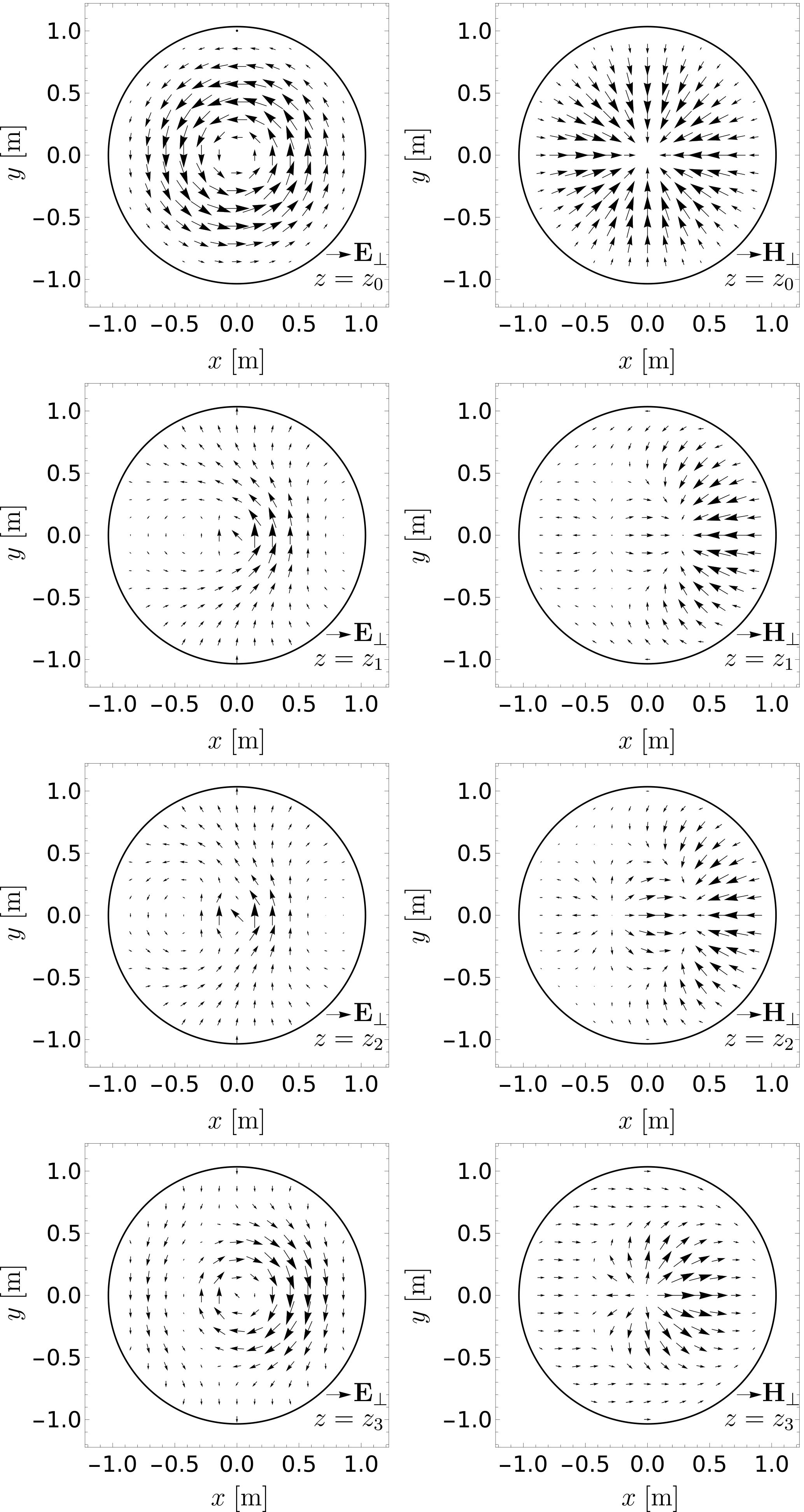
Figure 3Change of transverse field pattern of the electric and magnetic field along the z-axis. Parameters for simulation: N=60, r₀=1 and ${\mathit{\delta }}_{max}=\mathrm{1}$.

Download

In this section, we will present the method of computing the stochastic GTE's. After substituting the field components of the IBC Eq. (25) into each integrand of the line integrals of Eqs. (16) and (17), the coupling coefficients on the right side of the equations will be divided into a deterministic and stochastic part. Combining the Eqs. (16) and (17) into the form of state space equations we obtain

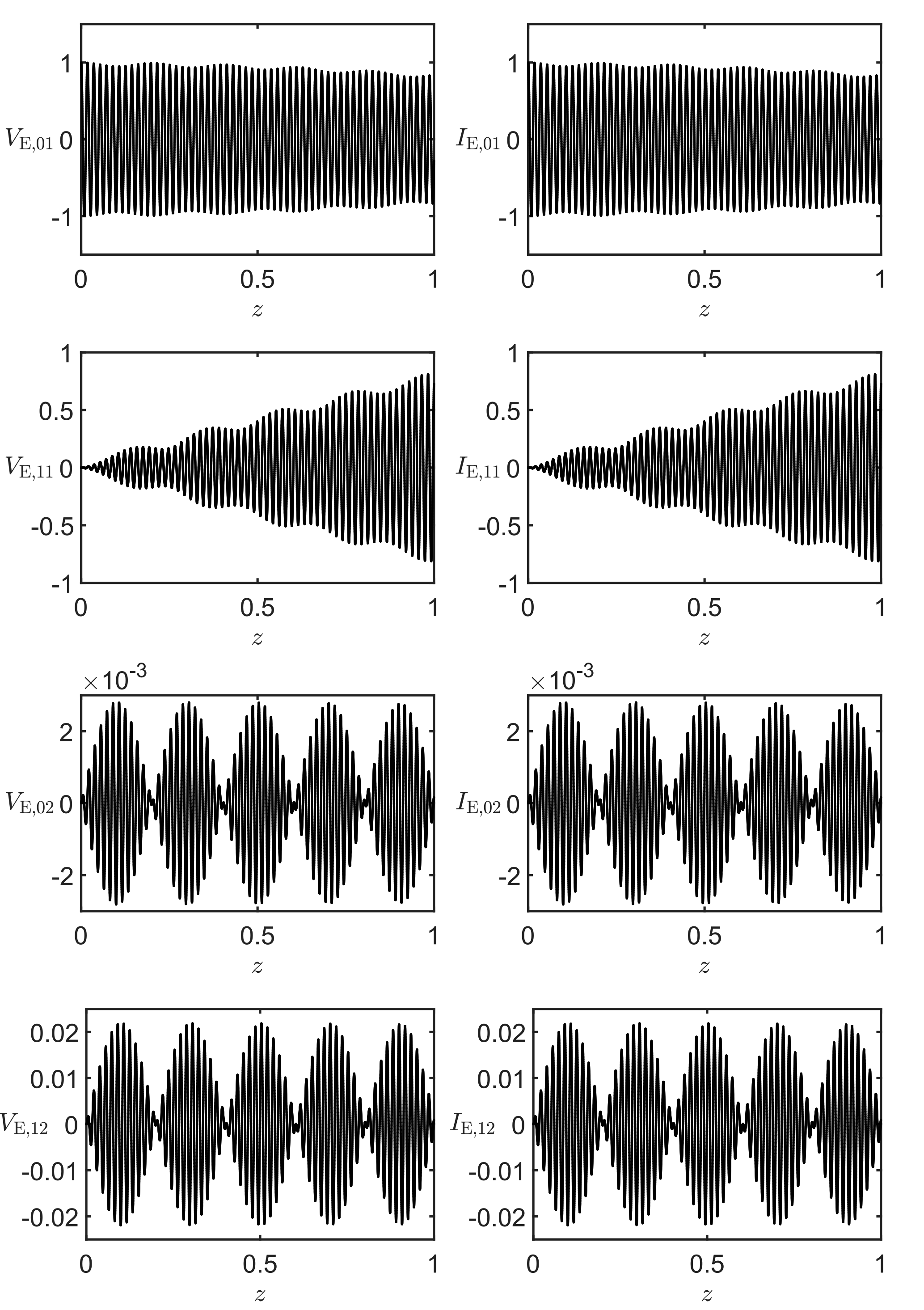
Figure 4All the basis coefficients V_E,n and I_E,n. Parameters for simulation: N=60, r₀=1 and ${\mathit{\delta }}_{max}=\mathrm{1}$.

Download

Table 2Parameters for simulation of excited TE₀₁-mode.

Download Print Version | Download XLSX

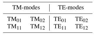
The next task is to consider all couplings between the different modes (see Table 1). For convenience, the double subscription for the designation of various modes has been substituted by a single subscription, but in order to consider all possible couplings the double subcription is useful. We will substitute the single subscription n and m with the double subscription [pq] and [rs]

In the case of the introduced stochastic process X(ϕ,ω) (Eq. 26), the matrices $\underset{\mathrm{¯}}{\mathbf{D}}$ and $\underset{\mathrm{¯}}{\mathbf{S}}$ (Eq. 28) become sparse matrices

As an example, we will calculate the basis coefficients V_n,I_n for an excited TE₀₁-mode. The simulation parameters are shown in Table 2. δ_max describes the maximum deviation from the mean radius r₀, while z_i characterizes four different cross-sections of the waveguide. The associated voltage and currents coefficients V_n,I_n are shown in Fig. 4. In Fig. 3, there are the transverse patterns of the electric and magnetic field at four different cross-sections. There are obvious changes of the transverse pattern due to the variation of the radius (see Fig. 1). In the case of a TE₀₁-mode, the electric and magnetic field components are

The deformation causes other field components to arise, which can be seen in the changes of the transverse pattern of the electric and magnetic field (see Fig. 3). According to the results of the simulation for the voltage and current coefficients, there is an attenuation to V_M,01 and I_M,01, besides the excited TE₀₁-mode there are other spurious modes (see Fig. 4). If the maximal deviation become less than 0.1 % of the mean radius r₀, the transverse pattern of the electric and magnetic field show no significant changes along the propagation direction (see Fig. 2). It is also important to mention that the impedance factor Z (Eq. 24) is restricted to small values close to Z=0 (Botton et al., 1998; Vlasov and Antonsen, 2001). The effect of mode conversion and attenuation of the excited wave will not be discussed in this work and need further investigation.

There are no underlying research data for the presented work. All results can be reproduced with the equations and parameters given directly in the paper.

The authors declare that they have no conflict of interest.

This article is part of the special issue “Kleinheubacher Berichte 2017”. It is a result of the Kleinheubacher Tagung 2017, Miltenberg, Germany, 25–27 September 2017.

The publication of this article was funded by the open-access
fund of Leibniz Universität Hannover.

Edited by: Thomas Eibert
Reviewed by: two anonymous referees