 | 04 Sep 2018
Delayed response of the ionosphere to solar EUV variability
Jens Berdermann
Norbert Jakowski
Christoph Jacobi
Rajesh Vaishnav
Physical and chemical processes in the ionosphere are driven by complex interactions with the solar radiation. The ionospheric plasma is in particular sensitive to solar EUV and UV variations with a time delay between one and two days. This delay is assumed to be related to thermospheric transport processes from the lower ionosphere to the F region. In previous analyses, the delay has been investigated using the F10.7 index. Here we present preliminary results of the ionospheric delay based on a comprehensive and reliable database consisting of GNSS TEC Maps and EUV spectral flux data. We plan to specify the various dependencies from geographic/geomagnetic location, altitude, season, local time, geophysical and solar radiation conditions such as the solar activity level. The first results for dependencies from seasons and wavelengths regions of the EUV are presented in this paper. These results can provide more insight into ionospheric processes and are of interest for applications dependent on reliable ionospheric weather forecasts, e.g. GNSS error analyses, prediction and mitigation.


The high variability of the ionospheric plasma has a strong influence on the radio signal propagation and therefore an impact e.g. on all applications based on Global Navigation Satellite Systems (GNSS), like navigation support, traffic guidance systems, land survey and communication services. Therefore, understanding the processes of the solar-ionosphere interaction, as a crucial source of the high dynamics of the ionosphere, is not only of interest for scientists, but also for engineers and service operators. The ionospheric ionization depends on the solar radiation intensity in combination with the recombination rate and transport processes due to diurnal, seasonal and geographic variations. The solar EUV radiation dominates the photoionization in the ionosphere and causes different variations like the 27-day solar rotation cycle or seasonal changes. The impact of the solar EUV radiation depends on the wavelength together with the absorption and ionization cross-sections of the varying particle populations at different heights, which cause a chain of reactions on different time scales with impact on the plasma structure of the ionosphere.
The different ionospheric layers are characterized by the density distribution of the different atom and molecule species. The understanding of the influence of solar radiation on the ionosphere and a potential delay in plasma production is essential for the development of realistic ionospheric models, having the potential to allow a precise prediction of the ionosphere with high spatial and temporal resolution. In the past investigations of the ionospheric delay were frequently based on the F10.7 index as proxy for the EUV variability (Jakowski et al., 1991). The observational results were further investigated by modeling the thermospheric response to the solar radiation variation using a one-dimensional numerical model between 100 and 250 km height. The simulation revealed a delayed density variation of atomic oxygen of about two days at 180 km height due to photodissociation. Jakowski et al. (1991) have introduced several simplifying assumptions such as a fixed thermosphere temperature profile, limitation to O and O2 thermospheric constituents and a fixed downward flow of atomic oxygen at the lower boundary. Here it is expected that thermosphere-ionosphere coupling plays a significant role for the delayed response of the ionospheric ionization.
The reason why F10.7 has been used as a proxy in the earlier analysis was due to a lack of direct EUV measurement in the relevant spectrum range. A delay between one and two days was confirmed by others using F10.7 and EUV proxies to describe the solar radiation correlation with the total electron content (TEC) (Oinats et al., 2008; Kutiev et al., 2013). The delay was also measured by using different indices for the solar radiation. Studies by Vellante et al. (2009) have indicated that the delay appears even in the plasmaspheric electron density derived from cross-spectral analyses of ULF wave measurements recorded at ground magnetometer stations. Thus, the delayed response of ionosphere/plasmasphere ionization to mid-term solar irradiance changes (variation within days, e.g. induced by the solar rotation) has a fundamental character which requires more exploration. In order to analyse the radiation effect on the ionospheric plasma, the TEC can be used as indicator for the ionization of the F region and ionosphere in general. Variations in the EUV radiation (like the 27-day cycle or seasonal changes) cause variations of TEC. To improve future ionosphere modelling a more detailed explanation of the delay with higher temporal and spectral resolution of the data and also consideration of different locations is needed.
In this paper we will give more insight by comparing the ionospheric delay to ionization, photodissociation and recombination processes respectively, as well as short term and long term seasonal and solar changes.
Nowadays, data of the solar spectrum in the EUV wavelength are available for more than one decade from the Solar EUV Experiment (SEE) onboard the Thermosphere Ionosphere Mesosphere Energetics and Dynamics (TIMED) satellite (Woods et al., 2005), and from the Solar Dynamics Observatory (SDO) (Woods et al., 2012) experiment. The SDO is a mission launched by the NASA in 2010 that has several instruments onboard: Extreme Ultraviolet Variability Experiment (EVE), Helioseismic and Magnetic Imager (HMI) and Atmospheric Imaging Assembly (AIA). The EVE instrument measures the solar EUV radiation in a wavelength region from 0.1 to 105 nm with a spectral resolution of 0.1 nm; it has a temporal resolution of 20 s and achieves an accuracy of 25 % with the inflight calibration (Woods et al., 2012). A high temporal resolution is available for the Geostationary Operational Environmental Satellites (GOES) data (Machol et al., 2014), but these are only available for several data bands in the EUV range. The available wavelength regions are from 5 to 15 nm, 25 to 35 nm and 115 to 130 nm. The GOES data have a temporal resolution of 1 min (Machol et al., 2014). A specific experiment to measure EUV spectral solar radiance calibrated in flight is Solar Auto-Calibrating EUV/UV Spectrophotometers (SolACES) (Schmidtke et al., 2006, 2014; Nikutowski et al., 2010) as a part of the ESA SOLAR ISS mission. Generally, the time resolution of the available data is 1 day, but due to ISS maneuvers there are repeated gaps. Therefore, SolACES data are not useful for time series analyses, but can be applied to calibrate regular observations from TIMED/SEE or SDO/EVE.
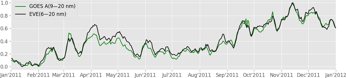
The SDO/EVE and GOES data are best suited for the analysis in this paper, because of the high temporal and spectral resolution and length of the missions. The integrated EUV of a wavelength region in EVE and the corresponding GOES band show a good correlation, as can be seen in Fig. 1. The other EUV data are not considered because of the mentioned deficiencies.
In the analysis, the EUV data will be compared with TEC values extracted from TEC maps provided by the International GNSS Service (IGS) TEC maps (Hernández-Pajares, 2004; Hernández-Pajares et al., 2009). TEC is the preferred parameter to investigate the solar dependence of ionospheric ionization, because TEC is an integral measurement of the electron density and therefore not as sensitive to vertical redistribution of plasma as for example the peak electron density. Furthermore, the good coverage and 24/7 operationality of ground based GNSS reference stations used for TEC calculation allow a permanent, high resolution and global access to the TEC parameter. The correlation with the solar EUV radiation can be calculated at single locations or regions. The time periods of the analysis are chosen to avoid big data gaps and to guarantee a minimal impact of small remaining gaps on the calculation of the delay.
2.1 Correlation between F10.7 and TEC
The delay between one to two days of solar EUV radiation and ionospheric parameters has been shown with the solar index F10.7 by Jakowski et al. (1991). Unglaub et al. (2011) and Jacobi et al. (2016) confirmed the delay with the EUV-TEC, which is calculated from satellite-born EUV measurements and represents the ionospheric variability better than the conventional F10.7 does. Since EUV-TEC does not account certain effects (e.g. secondary ionization), the same delay was also calculated with EVE fluxes by Jacobi et al. (2016).
In Fig. 2 we could reproduce the results via the calculation of the cross-correlation between F10.7 and TEC. In the left plot in Fig. 2 the normalized (feature scaling) F10.7 and TEC data are shown. In the calculation of the TEC map correlation data from the grid point 50∘ N and 10∘ E are used, since this position is in a region with a high number of ground stations and thus the data strongly rely on real measurements. In addition the TEC data have been resampled to a resolution of 1 day because the F10.7 data are not available in a higher resolution. The resulting cross-correlation of F10.7 and TEC is shown in the middle plot of Fig. 2. In the right plot of Fig. 2 the peak of the correlation is given, indicating a delay of about one day between F10.7 and TEC.
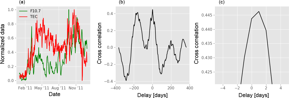
Figure 2Comparison of normalized F10.7 and TEC (for grid point 50∘ N, 10∘ E), cross-correlation of F10.7 and TEC, peak of the cross-correlation of F10.7 and TEC. The middle plot shows, that the peak and delay can be estimated from the entire cross-correlation for the given time period and resolution without making assumptions about an expected value.
Further calculations show that the estimated delay varies between one and two days for the analyzed years (2011: 1 day, 2012: 1 day, 2013: 1 day, 2014: 2 days and 2015: 2 days). Due to the daily resolution of F10.7 the calculation of the delay for different regions does not show any significant variations and a more precise calculation of the delay is not possible here. Therefore we apply in the next section the same correlation process to the higher temporal resolution of the nowadays available EUV data.
2.2 Correlation between EUV and TEC
For the calculation of the cross-correlation between EUV and TEC also the TEC data used were adjusted to a temporal resolution of 1 h. A band-stop filter using fast Fourier transform from 23 to 25 h is applied to remove the daily variability. The EVE data are integrated over 3 to 100 nm to get a single data series representing the EUV radiation in the correlation.

Figure 3Comparison of normalized integrated EUV (EVE from 3 to 100 nm) and TEC (for grid point 50∘ N, 10∘ E) for summer, cross-correlation of integrated EUV and TEC, peak of the cross-correlation of integrated EUV and TEC. The middle plot shows, that the peak and delay can be estimated from the entire cross-correlation for the given time period and resolution without making assumptions about an expected value.
Figure 3 shows the comparison and cross-correlation for the integrated EUV and the TEC values from the grid point 50∘ N and 10∘ E. The left plot in Fig. 3 shows a delay of about 16 hours for a chosen time period during the summer season. A cross-correlation for a shorter time period is compared to the earlier results, because there are no gaps in the data and therefore no interpolations had to be applied. For a rough comparison of the correlations between F10.7 and TEC and also EUV and TEC this approach is sufficient. The calculated delay is in agreement with the rough delay of one day estimated with the F10.7 index around this time period. Therefore it is possible to reproduce earlier results with much higher precision by using recent EUV measurements. The variation of the delay between one and two days estimated with the F10.7 index and a similar behavior for the estimation with EUV, as shown in Fig. 5, is discussed in the further analysis.
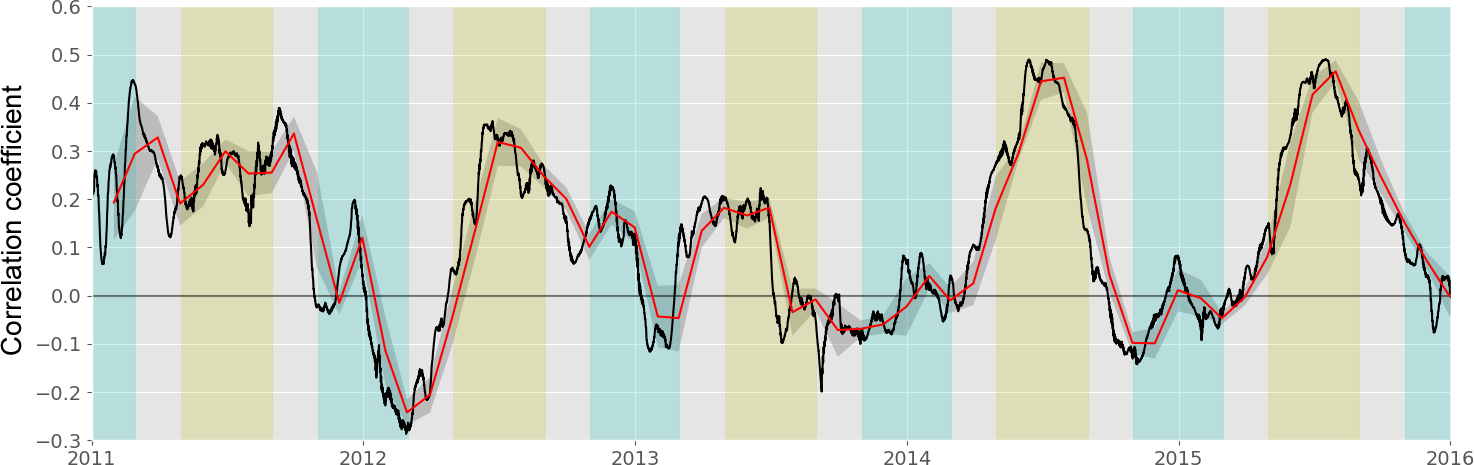
Figure 4Running correlation coefficients (window of 90 days) of EUV (GOES E from 115 to 130 nm) and TEC (for grid point 50∘ N, 10∘ E). The red line and grey shading are the mean and standard deviation for each month of the year. Summer and winter months are shaded in yellow and blue.
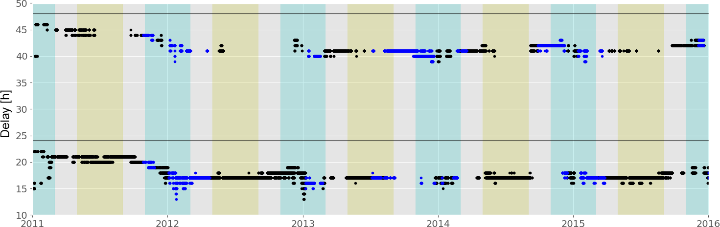
Figure 5Delay of EUV (GOES E from 115 to 130 nm) and TEC (for grid point 50∘ N, 10∘ E). The blue dots represent delays which are related to negative correlations. Summer and winter months are shaded in yellow and blue.
In order to analyse a possible seasonal effect on the delay, which might be caused by a seasonal dependence of ionospheric dynamics and photodissociation, the analysis needs to be further improved and consider more than a single time period. Figures 4 and 5 show a time series of the correlation coefficient and the delay for a period of 5 years, where each point is calculated for a time window of 90 days. This time window is applied, because it is long enough to result in reliable cross-correlations for the delay estimation and because it is short enough to allow capturing changes in the delay over time. Here we used EUV data from GOES E for the comparison with TEC data at the grid point 50∘ N and 10∘ E because they cover the longest time period of continuous EUV data measurement.
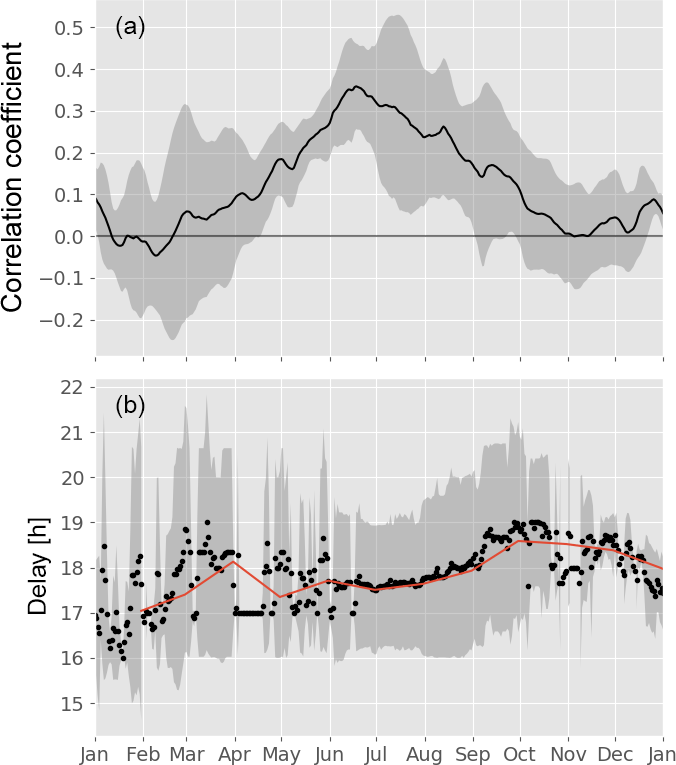
Figure 6Super epoch analysis of the correlation coefficient and delay from 2011 to 2015 with EUV (GOES E from 115 to 130 nm) and TEC (for grid point 50∘ N, 10∘ E). In the upper plot the black line and grey shading are the mean and standard deviation of the correlation coeffecient for each day. In the lower plot the black dots and grey shading are the mean and standard deviation of the delay for each day; the red line is the mean of the delay for each month.
The correlation of EUV and TEC in Fig. 4 shows an increase in summer and a decrease in winter, although the correlation is slightly different in each summer and winter. The annual difference might be caused by changes in the EUV radiation due to the solar cycle or peculiarities of the thermospheric dynamics in different years. In some winter periods the correlation reaches negative values and the corresponding delays have been highlighted in Fig. 5 in order to show that the delay's deviation is increased. The delay itself, as visible in Fig. 5, is grouped in two peaks below 24 and 48 h. This clustering is caused by the one day variation of the TEC data, which induces a similar variation in the cross-correlation results. By comparing both groups we find that the values around 48 h have many gaps and belong mostly to a negative correlation. In addition the number of cross-correlation maxima around 24 h outnumbers the results around 48 h by a factor of 3. We believe that the second band at 48 h is caused by the maximum of the cross-correlation which sometimes originates from a pronounced second peak, which cannot be removed completely with the above mentioned band-stop filter. Therefore, we expect that values which belong in the group around 24 h represent the actual delay and we disregard all other values in the further analysis.
As can be seen in Fig. 5, the delay decreases for a few hours in winter and increases again during summer. There also seems to be an overall trend which lets the delay decrease slightly in the middle of the chosen time period. To allow a better comparison of the seasonal variation, the results of Fig. 5 are used to calculate the super epoch plots in Fig. 6, which shows the mean trend of the correlation and delay through the seasons.
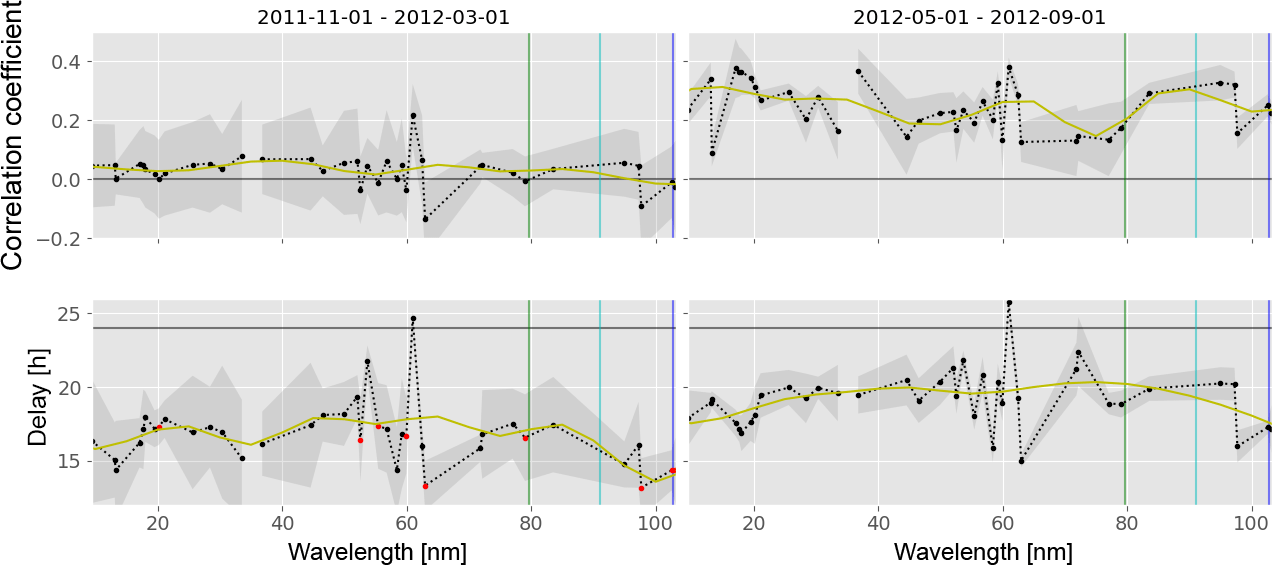
Figure 7Correlation and delay of EUV (EVE) and TEC (for grid point 50∘ N, 10∘ E) for a summer and winter period. Red dots are delays which are related to negative correlations. Green line: Start of N2 ionization, cyan line: start of O ionization, blue line: start of O2 ionization.
Comparing the seasonal values in the years from 2011 to 2015 the correlation in the upper plot of Fig. 6 reaches its maximum in the month June and have their minimum in February. The mean value of the correlation varies from in Winter to ≈0.35 in Summer. The increase and decrease of the delay (Fig. 6 lower plot) seems to be slower with a maximum shifted to October and a minimum shifted from January to February. This could be an indication that atmospheric processes might have an additional influence on the ionospheric delay. The mean value of the delay varies between 17 to 18.5 h for winter and summer respectivly. The slower and delayed increase of the delay shown in the lower plot of Fig. 6 compared to the correlation coefficient in the upper plot of Fig. 6 indicates that there are processes involved which are not directly related to the EUV radiation. These effects (e.g. transport processes or coupling with the lower atmosphere) must be stronger in winter and cause the decreased correlation between EUV and TEC. We expect that seasonal changes of thermospheric winds might be a candidate of such additional process responsible for the smaller seasonal variations in the delay.
To further analyse the variation between different EUV spectral bands we compare the whole wavelength spectrum available from EVE data in Fig. 7, instead of using the integrated EUV data.
For a detailed view of the spectral bands the ionization potentials of N2, O and O2 are added in Fig. 7, which absorb most of the EUV radiation at different spectral bands in the F region of the ionosphere. A detailed view of the ionization cross sections is shown in Fig. 8. The correlation and delay are again much stronger in summer than in winter for every investigated wavelength. There is also a profile of the correlation and delay that is similar in every of the chosen time periods with a maximum at ≈62 nm. The wavelengths at which the different ionizations begin do not show any noticeable variations. Therefore the delay to 24 h is similar for most wavelengths, but has a slight increase around the above-mentioned maximum. The contribution of the ionizations of each species to the delay cannot be estimated with the given results because most of the EUV variability at different wavelengths is correlated. This causes a very similar behaviour for the whole EUV spectrum.
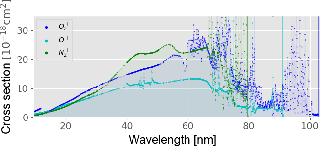
Figure 8Ionization cross sections of N2, O and O2. Green line: start of N2 ionization, cyan line: start of O ionization, blue line: start of O2 ionization (Fennelly et al., 1992).
As seen in Fig. 8, the ionization profiles of N2, O and O2 have their maximums similar to the trend of the delay through the wavelength spectrum, but no reliable correlation can be estimated with the given data.
With the analysis of EUV and TEC data the earlier results from Jakowski et al. (1991) or Jacobi et al. (2016) were confirmed and calculated with more precision. The calculated delay is about ≈17 h on an average during a year. The difference to 24 h indicates that besides the seasonal and daily variation other effects in the ionosphere contribute to the delay. In the overall trend of the delay in Fig. 5 a small decrease in the middle of the five years can be seen. This might be the influence of the solar cycle which shows the same trend for this time period. Similar to the seasonal variation an increase of the EUV radiation and therefore of the ionization could cause a stronger correlation and delay. Further analysis for longer time periods that include solar maximums and minimums are necessary to show if such an effect exist. The higher resolution of the delay calculation also showed the seasonal variation of the correlation and delay. The seasonal variation was calculated using GOES and SDO/EVE data. The decrease of the correlation in winter shows that the influence of the ionization is slightly reduced, which allows other effects to have a visible impact on the delay, causing the resulting seasonal variation in the delay. The shift between the maximum of the EUV-TEC correlation compared to the maximum of the ionospheric delay in late summer also indicates the influence of other effects. The coupling with the seasonal variations of thermospheric winds might be a candidate having some influence on the delay. This needs to be investigated in more detail in a future work. Furthermore, the analysis of EUV and other ionospheric parameters besides TEC (e.g. hmF2 or NmF2) needs to be done in future work, to investigate if a similar or different delay could give more insight into the physics of the seasonal variation. The possible effects of the ionization of different species were analysed by correlating the whole EUV spectrum with the TEC data. It could be shown that the different wavelengths bands of EUV have no major impact on the correlation and delay. The whole EUV spectrum is contributing in the same order of magnitude to the delay.
In future analysis also the UV data should be added, which allows to take the photodissociation into account which happens around ≈150 nm. Such an analysis could confirm the influence on the delay by atomic and molecular oxygen mentioned in Jakowski et al. (1991) and Jacobi et al. (2016). The results indicate that photodissociation processes might be primarily cause for differences in the delay. The coupling with thermospheric winds (Chen et al., 2014) is expected to have some influence too, but needs to be investigated in more detail in future. Although ionization processes are crucial for the genesis of the ionosphere, their influence on the ionospheric delay has to be analyzed for the different ionospheric reactions in the F region. Another major point of interest for future analysis is the dependence of the delay from longitude and latitude. In this paper all calculations used the same location and focused on the dependence on wavelengths and time.
IGS TEC maps has been provided by NASA through (ftp://cddis.gsfc.nasa.gov/gnss/products/ionex/). F10.7 data has been provided by NASA through (ftp://spdf.gsfc.nasa.gov/pub/data/omni/). EVE data has been provided by LASP through (http://lasp.colorado.edu/eve/data_access/evewebdata/products/level3/, Tapping, 2013). GOES data has been provided by NOAA through (https://satdat.ngdc.noaa.gov/sem/goes/data/euvs/).
The authors declare that they have no conflict of interest.
This article is part of the special issue “Kleinheubacher Berichte 2017”. It is a result of the Kleinheubacher Tagung 2017, Miltenberg, Germany, 25–27 September 2017.
IGS TEC maps and F10.7 data have been provided by NASA. GOES data has been
provided by NOAA. EVE data has been provided by LASP. The study has been
supported by Deutsche Forschungsgemeinschaft (DFG) through grants no. BE 5789/2-1 and JA 836/33-1.
Edited by: Ralph
Latteck
Reviewed by: Ljiljana R. Cander and one anonymous
referee
Chen, Y., Liu, L., Le, H., and Wan, W.: How does ionospheric TEC vary if solar EUV irradiance continuously decreases?, Earth Planet. Space, 66, 52 pp., https://doi.org/10.1186/1880-5981-66-52, 2014. a
Fennelly, J. A. and Torr, D. G.: Photoionization and photoabsorption cross sections of O, N2, O2, and N for aeronomic calculations, Atom. Data Nucl. Data Tables, 51, 321–363, https://doi.org/10.1016/0092-640X(92)90004-2, 1992.
Hernández-Pajares, M.: IGS Ionosphere WG Status Report: Performance of IGS Ionosphere TEC Maps Position Paper, 263–275, 2004. a
Hernández-Pajares, M., Juan, J. M., Sanz, J., Orus, R., Garcia-Rigo, A., Feltens, J., Komjathy, A., Schaer, S. C., and Krankowski, A.: The IGS VTEC maps: a reliable source of ionospheric information since 1998, J. Geodesy, 83, 263–275, https://doi.org/10.1007/s00190-008-0266-1, 2009. a
Jacobi, C., Jakowski, N., Schmidtke, G., and Woods, T.: Delayed response of the global total electron content to solar EUV variations, Adv. Radio Sci., 14, 175–180, https://doi.org/10.5194/ars-14-175-2016, 2016. a, b, c, d
Jakowski, N., Fichtelmann, B., and Jungstand, A.: Solar activity control of ionospheric and thermospheric processs, J. Atmos. Terr. Phys., 53, 1125–1130, https://doi.org/10.1016/0021-9169(91)90061-B, 1991. a, b, c, d, e
Kutiev, I., Tsagouri, I., Perrone, L., Pancheva, D., Mukhtarov, P., Mikhailov, A., Lastovicka, J., Jakowski, N., Buresova, D., Blanch, E., Andonov, B., Altadill, D., Magdaleno, S., Parisi, M., and Torta, J. M.: Solar activity impact on the Earth's upper atmosphere, J. Space Weather Space, 3, A06, https://doi.org/10.1051/swsc/2013028, 2013. a
Machol, J., Viereck, R., and Jones, A.: GOES EUVS Measurements, v2. https://www.ngdc.noaa.gov/stp/satellite/goes/doc/GOES_NOP_EUV_readme.pdf (last access: 22 November 2017), 2014. a, b
Nikutowski, B., Brunner, R., Jacobi, C., Knecht, S., Ehrhardt, C., and Schmidtke, G.: EUV measurements by the auto-calibrating SolACES spectrometers onboard the International Space Station (ISS), 7 pp., 2010. a
Oinats, A. V., Ratovsky, K. G., and Kotovich G. V.: Influence of the 27-day solar flux variations on the ionosphere parameters measured at Irkutsk in 2003–2005, Adv. Space Res., 42, 639–644, https://doi.org/10.1016/j.asr.2008.02.009, 2008. a
Schmidtke, G., Brunner, R., Eberhard, D., Halford., B., Klocke, U., Knothe, M., Konz, W., Riedel, W.-J., and Wolf, H.: SOL-ACES: Auto-calibrating EUV/UV spectrometers for measurements onboard the International Space Station, Adv. Space Res., 37, 273–282, https://doi.org/10.1016/j.asr.2005.01.112, 2006. a
Schmidtke, G., Nikutowski, B., Jacobi, C., Brunner, R., Erhardt, C., Knecht, S., Scherle, J., and Schlagenhauf, J.: Solar EUV irradiance measurements by the Auto-Calibrating EUV Spectrometers (SolACES) aboard the International Space Station (ISS), Sol. Phys., 289, 1863–1883, https://doi.org/10.1007/s11207-013-0430-5, 2014. a
Tapping, K. F.: The 10.7 cm solar radio flux (F10.7), Space Weather, 11, 394–406, https://doi.org/10.1002/swe.20064, 2013.
Unglaub, C., Jacobi, Ch., Schmidtke, G., Nikutowski, B., and Brunner, R.: EUV-TEC proxy to describe ionospheric variability using satellite-borne solar EUV measurements: first results, Adv. Space Res., 47, 1578–1584, https://doi.org/10.1016/j.asr.2010.12.014, 2011. a
Vellante, M., Förster, M., Pezzopane, M., Jakowski, N., Long Zhang, T., Villante, U., De Lauretis, M., Zolesi, B., and Magnes, W.: Monitoring the Dynamics of the Ionosphere-Plasmasphere System by Ground-Based ULF Wave Observations, Earth Moon Planets, 104, 25–27, https://doi.org/10.1007/s11038-008-9246-y, 2009. a
Woods, T. N., Eparvier, F. G., Bailey, S. M., Chamberlin, P. C., Lean, J., Rottman, G. J., Solomon, S. C., Tobiska, W. K., and Woodraska, D. L.: Solar EUV Experiment (SEE): Mission overview and first results, J. Geophys. Res., 110, A01312, https://doi.org/10.1029/2004JA010765, 2005. a
Woods, T. N., Eparvier, F. G., Hock, R., Jones, A. R., Woodraska, D., Judge, D., Didkovsky, L., Lean, J., Mariska, J., Warren, H., McMullin, D., Chamberlin, P., Berthiaume, G., Bailey, S., Fuller-Rowell, T., Sojka, J., Tobiska, W. K., and Viereck, R.: Extreme Ultraviolet Variability Experiment (EVE) on the Solar Dynamics Observatory (SDO): Overview of Science Objectives, Instrument Design, Data Products, and Model Developments Solar Physics, 275, 115–143, https://doi.org/10.1007/s11207-009-9487-6, 2012. a, b